Excel Bubble Sort - Arranging Many Cells in Many Columns

In a previous post, and to some extent in a later one, I worked on ways to sort Excel cells in which data started out in an irregular arrangement, like this:

My goal in that case was to get the data items arranged in the original (vertical) order in a single column, like this:

This time around, I had a somewhat different objective. It seemed likely to require me to continue past the outcome just shown, to return the data to their original columns, but without the empty spaces between them, like this:

The question for this post was, how would I do that?

As I reviewed the previous posts, it seemed that the key step was to use Excel's CELL function. In the example just shown, an adjacent table containing formulas like =CELL("address",A1) and =CELL("address",A2) would produce values like $A$1 and $A$2. I could make those formulas conditional. Then =IF(A3="","",CELL("address",A3)) would return a blank cell. One additional step: I could combine the cell's address and its contents, like this:

The formula for that was =IF(A1="","",CELL("address",A1)&"--"&A1).  Now I could set up a shadow table, matching the original one cell for cell, with the same number of rows and columns, and with each cell containing this kind of CELL formula.  

With that done, I could copy the parallel table to a word processor that would have the ability to remove line breaks.  (The find-and-replace symbol for a line break in Microsoft Word was usually ^p.)  The table I was working on had 100 columns and about 3,000 rows.  Each column had just 30 actual data items, so there were a total of exactly 3,000 (not 300,000) actual data items in that table; all the other cells were blank.  Word 2003 was not able to accommodate this table initially, so I pasted it into Notepad++ and saved it as a text file, and then opened that in Word.  After a series of find-and-replace operations (replacing double tabs (i.e., ^t^t) and so forth), I wound up with a single column of entries, 53 pages long.

I pasted that list back into a different Excel table, temporarily, for further operations.  I parsed the entries into separate columns, using FIND to divide each item into its address and its contents.  In the first cell shown in the example above, the address was $A$1 and the contents were 3.  Now I had the 30 items that had originally been in column A, the 30 items that had been in column B, and so forth, without any of those blank cells.  This resulting set of 3,000 items was  all still just in one long column, but I could sort them in column order; I could take another few steps and sort them in row order; or I could sort them by increasing data item value.

So at that point, I had achieved approximately what I had tried to do in at least one of the preceding posts.  Now there was the additional step of getting the 30 items pertaining to column A back into column A, leaving me with a table 100 columns wide but only 30 (not 3,000) rows deep.  To do this, I did go ahead and isolate out the column and row information into separate columns.  It was awkward to put the Excel column letters into proper order -- getting AA after Y, and so forth -- so I set up another column with numbers as substitute column indicators.  To do that, I did a unique data filter to get just a single representative from each column (e.g., AA, AB, ...), and then did a VLOOKUP to the appropriate number in a table built from that unique filter (e.g., Y = 1, Z = 2, AA = 3 ...).  This gave me a table which, after sorting, began like this:

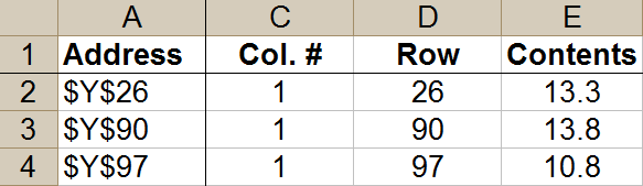
I further modified this table by adding a Row # column after the existing Row column.  For this project, I didn't care what row the item came from in the original spreadsheet; I just cared that it was sorted in proper row order and that it would appear somewhere within rows 1-30 of my new table.  So the numbers in this new Row # column just ran from 1 to 30, matching the 30 items from a given column in the original spreadsheet (e.g., Y), and then they started over again at 1 and ran up to 30 for the next original column (e.g., Z), and so forth).  This was easy enough to arrange:  after setting up the first set of 1 to 30, the cells in all following rows could just refer to the value appearing 30 rows up.  So now I had set of 1, 2, 3 ... 30, appearing over and over again, all the way down my new Row # column.  I added a new NAddress column to express the combination of row and column: 

With that in place, I could do a lookup to complete the job.  This called for two tables.  The top left corners of those two tables looked like this:

Note the formulas shown for the top left data cell in each of these two tables.  The first table produced the thing that I would be looking for in my VLOOKUP; the second was the final data table.

I soon discovered that I should have included a VALUE formula in that final table's calculations; the resulting data were behaving like strings, not numbers, so I did have to do that additional transformation.  Otherwise, though, the data checked out OK, so this task was done.